library(tidyverse)
library(dplyr)
library(skimr)Project
beer market
library(ggplot2)
library(dplyr)


url <- "https://bcdanl.github.io/data/beer_markets_all.csv"
beer_markets <- read.csv(url)


beer_markets2 <- beer_markets |>
  group_by(state, brand) |>
  summarise(n = n()) |>
slice_max(n, n=10)skim(beer_markets)| Name | beer_markets |
| Number of rows | 73115 |
| Number of columns | 25 |
| _______________________ | |
| Column type frequency: | |
| character | 14 |
| logical | 6 |
| numeric | 5 |
| ________________________ | |
| Group variables | None |
Variable type: character
| skim_variable | n_missing | complete_rate | min | max | empty | n_unique | whitespace |
|---|---|---|---|---|---|---|---|
| X_purchase_desc | 0 | 1 | 12 | 29 | 0 | 115 | 0 |
| brand | 0 | 1 | 9 | 13 | 0 | 5 | 0 |
| container | 0 | 1 | 3 | 30 | 0 | 7 | 0 |
| market | 0 | 1 | 5 | 20 | 0 | 92 | 0 |
| state | 0 | 1 | 4 | 20 | 0 | 49 | 0 |
| buyertype | 0 | 1 | 4 | 7 | 0 | 3 | 0 |
| income | 0 | 1 | 5 | 8 | 0 | 5 | 0 |
| age | 0 | 1 | 3 | 5 | 0 | 4 | 0 |
| employment | 0 | 1 | 4 | 4 | 0 | 3 | 0 |
| degree | 0 | 1 | 2 | 7 | 0 | 4 | 0 |
| cow | 0 | 1 | 4 | 25 | 0 | 4 | 0 |
| race | 0 | 1 | 5 | 8 | 0 | 5 | 0 |
| tvcable | 0 | 1 | 4 | 7 | 0 | 3 | 0 |
| npeople | 0 | 1 | 1 | 5 | 0 | 5 | 0 |
Variable type: logical
| skim_variable | n_missing | complete_rate | mean | count |
|---|---|---|---|---|
| promo | 0 | 1 | 0.20 | FAL: 58563, TRU: 14552 |
| childrenUnder6 | 0 | 1 | 0.07 | FAL: 68109, TRU: 5006 |
| children6to17 | 0 | 1 | 0.20 | FAL: 58155, TRU: 14960 |
| microwave | 0 | 1 | 0.99 | TRU: 72676, FAL: 439 |
| dishwasher | 0 | 1 | 0.73 | TRU: 53258, FAL: 19857 |
| singlefamilyhome | 0 | 1 | 0.81 | TRU: 59058, FAL: 14057 |
Variable type: numeric
| skim_variable | n_missing | complete_rate | mean | sd | p0 | p25 | p50 | p75 | p100 | hist |
|---|---|---|---|---|---|---|---|---|---|---|
| hh | 0 | 1 | 17407721.61 | 11582147.34 | 2000235.00 | 8223438.00 | 8413624.00 | 30171315.00 | 30440718.00 | ▂▇▁▁▇ |
| quantity | 0 | 1 | 1.32 | 1.15 | 1.00 | 1.00 | 1.00 | 1.00 | 48.00 | ▇▁▁▁▁ |
| dollar_spent | 0 | 1 | 13.78 | 8.72 | 0.51 | 8.97 | 12.99 | 16.38 | 159.13 | ▇▁▁▁▁ |
| beer_floz | 0 | 1 | 265.93 | 199.52 | 12.00 | 144.00 | 216.00 | 360.00 | 9216.00 | ▇▁▁▁▁ |
| price_per_floz | 0 | 1 | 0.06 | 0.01 | 0.00 | 0.05 | 0.06 | 0.06 | 0.23 | ▃▇▁▁▁ |
beer_markets2 <- beer_markets |>
  group_by(income, dollar_spent) |>
  summarise(n = n())
average_spent_by_income <- beer_markets %>%
group_by(income) %>%
summarize(average_dollar_spent = mean(dollar_spent, na.rm = TRUE)) |>
mutate(income = factor(income,
levels = c("under20k",
"20-60k",
"60-100k",
"100-200k",
"200k+")))
ggplot(average_spent_by_income, aes(x = income, y = average_dollar_spent ))+
geom_point()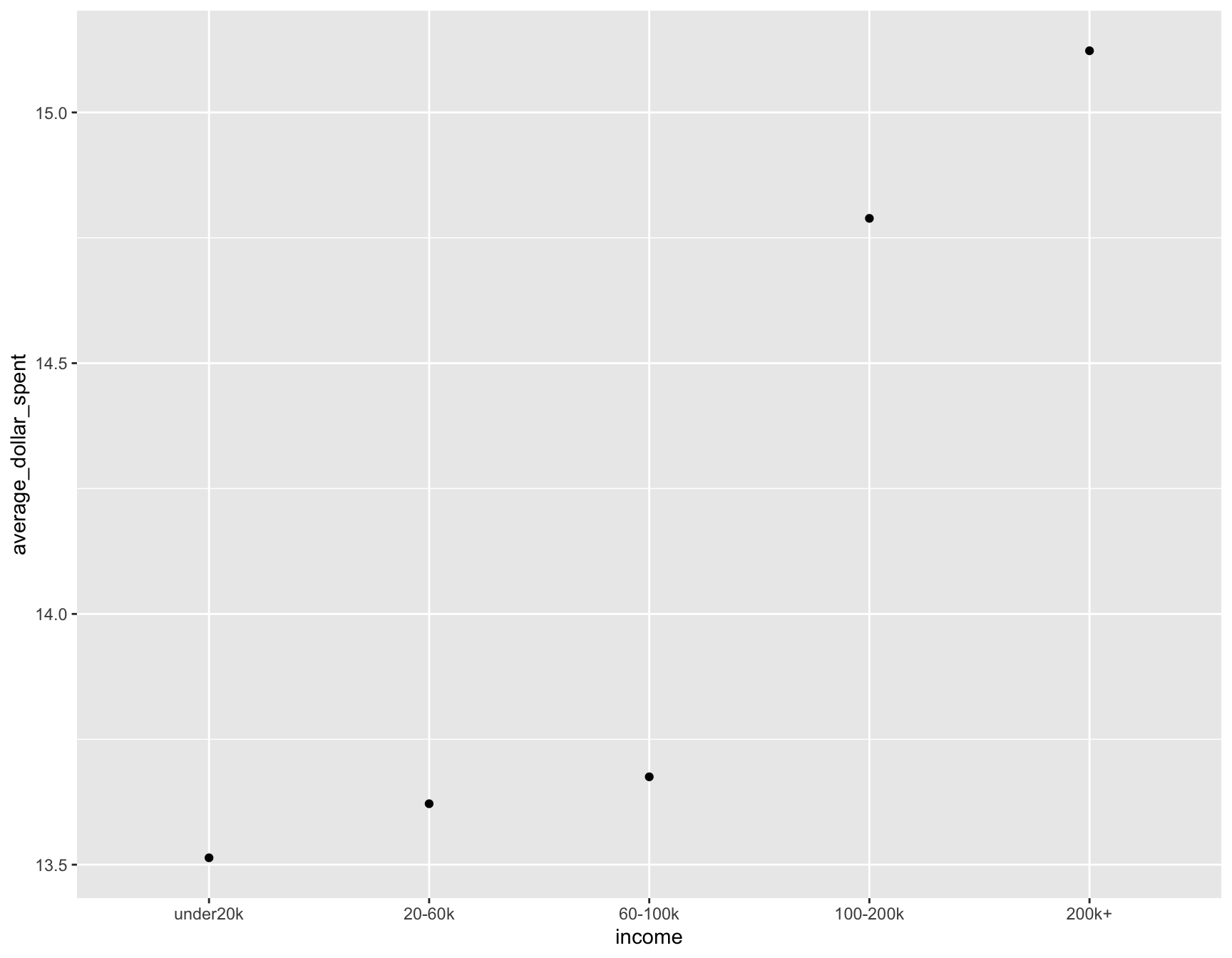
This graph is very interesting. It shows us how much each income bracket spends on average when purchasing beer. Unsurprisingly, the wealthier groups tend to spend more on average. What did surprise me though, is the fact that the lower income groups only spend around $2 less per purchase. It goes to show the difference in priorities between wealthy and poor people. Furthermore, this graph shows that alcohol consumption is something all income levels find important considering that they each spend similar amounts of money when buying alcohol.
beer_markets2 <- beer_markets |>
  count(state, income) |>
  group_by(state) |>
  mutate(total = sum(n)) |>
  ungroup() |>
  filter(dense_rank(-total)<=10) |>
  mutate(state = fct_reorder(state, total))

ggplot(beer_markets2)+
  geom_bar(aes(y = state, fill = income, x = n),
           stat = "identity", position = "fill")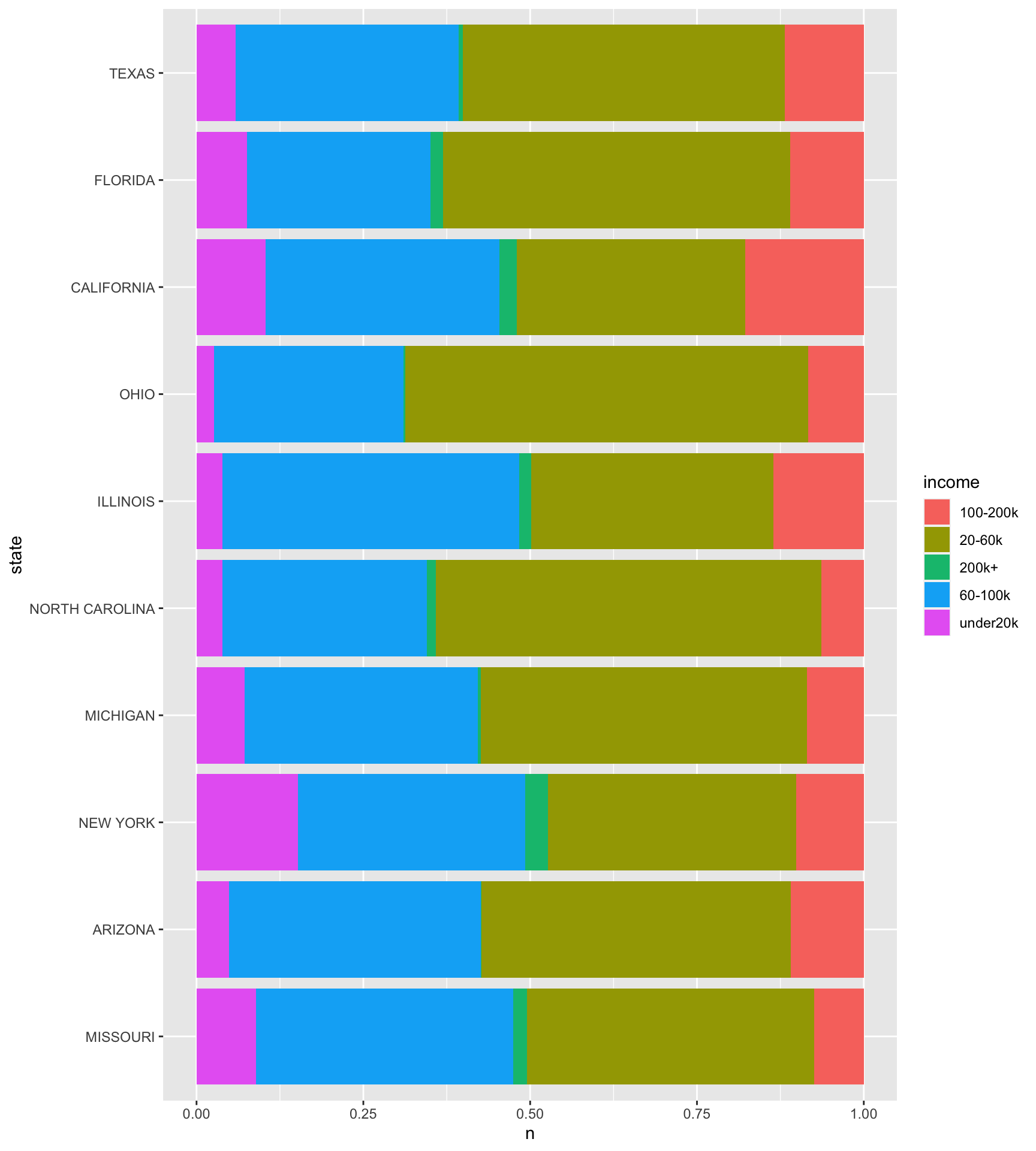
This graph shows the proportion of alcohol bought by each income group by state. In almost every state, the 20-60k group is spending the most on beer while the 200k+ group buys the least in every state observed. This is surprising because most people would expect that the people with the most money would buy the most beer. I think the reason for this is because people who are addicted to alcohol tend to have less money. The people who can control their usage are much more responsible with not only their drinking, but also their finances.